
Abstract
Detailed knowledge of the image of the point spread function (PSF) is necessary to optimize astronomical coronagraph masks and to understand potential sources of errors in astrometric measurements. The PSF for astronomical telescopes and instruments depends not only on geometric aberrations and scalar wave diffraction but also on those wavefront errors introduced by the physical optics and the polarization properties of reflecting and transmitting surfaces within the optical system. These vector wave aberrations, called polarization aberrations, result from two sources: (1) the mirror coatings necessary to make the highly reflecting mirror surfaces, and (2) the optical prescription with its inevitable non-normal incidence of rays on reflecting surfaces. The purpose of this article is to characterize the importance of polarization aberrations, to describe the analytical tools to calculate the PSF image, and to provide the background to understand how astronomical image data may be affected. To show the order of magnitude of the effects of polarization aberrations on astronomical images, a generic astronomical telescope configuration is analyzed here by modeling a fast Cassegrain telescope followed by a single 90° deviation fold mirror. All mirrors in this example use bare aluminum reflective coatings and the illumination wavelength is 800 nm. Our findings for this example telescope are: (1) The image plane irradiance distribution is the linear superposition of four PSF images: one for each of the two orthogonal polarizations and one for each of two cross-coupled polarization terms. (2) The PSF image is brighter by 9% for one polarization component compared to its orthogonal state. (3) The PSF images for two orthogonal linearly polarization components are shifted with respect to each other, causing the PSF image for unpolarized point sources to become slightly elongated (elliptical) with a centroid separation of about 0.6 mas. This is important for both astrometry and coronagraph applications. (4) Part of the aberration is a polarization-dependent astigmatism, with a magnitude of 22 milliwaves, which enlarges the PSF image. (5) The orthogonally polarized components of unpolarized sources contain different wavefront aberrations, which differ by approximately 32 milliwaves. This implies that a wavefront correction system cannot optimally correct the aberrations for all polarizations simultaneously. (6) The polarization aberrations couple small parts of each polarization component of the light (∼10-4) into the orthogonal polarization where these components cause highly distorted secondary, or "ghost" PSF images. (7) The radius of the spatial extent of the 90% encircled energy of these two ghost PSF image is twice as large as the radius of the Airy diffraction pattern. Coronagraphs for terrestrial exoplanet science are expected to image objects 10-10, or 6 orders of magnitude less than the intensity of the instrument-induced "ghost" PSF image, which will interfere with exoplanet measurements. A polarization aberration expansion which approximates the Jones pupil of the example telescope in six polarization terms is presented in the appendix. Individual terms can be associated with particular polarization defects. The dependence of these terms on angles of incidence, numerical aperture, and the Taylor series representation of the Fresnel equations lead to algebraic relations between these parameters and the scaling of the polarization aberrations. These "design rules" applicable to the example telescope are collected in § 5. Currently, exoplanet coronagraph masks are designed and optimized for scalar diffraction in optical systems. Radiation from the "ghost" PSF image leaks around currently designed image plane masks. Here, we show a vector-wave or polarization optimization is recommended. These effects follow from a natural description of the optical system in terms of the Jones matrices associated with each ray path of interest. The importance of these effects varies by orders of magnitude between different optical systems, depending on the optical design and coatings selected. Some of these effects can be calibrated while others are more problematic. Polarization aberration mitigation methods and technologies to minimize these effects are discussed. These effects have important implications for high-contrast imaging, coronagraphy, and astrometry with their stringent PSF image symmetry and scattered light requirements.
Export citation and abstract BibTeX RIS
1. Introduction
In this section, we describe briefly the value of polarization measurements to stellar and exoplanet astronomical sciences, summarize polarization aberrations, discuss the physical optics of image formation in astronomical telescopes, and describe how modern telescopes introduce polarization aberrations.
1.1. Photopolarimetry
Polarization measurements of astronomical sources contain substantial astrophysical information. Many stars observed in the UV, Visible, and IR are thermal emitters and their radiation at the star is unpolarized except for a minority of stars with high magnetic fields. Hiltner (1950) and Mavko et al. (1974) showed that the asymmetry of aligned dipoles in interstellar matter selectively absorbs the thermal emission from background stars. Unpolarized radiation that scatters from planetary atmospheres and circumstellar disks can become partially polarized. When one polarization is preferentially absorbed over its orthogonal state, the unpolarized starlight becomes partially polarized. Clarke (2010) and Perrin (2009a, 2009b) provide a comprehensive review of the value of precision polarization measurements to general astrophysics. Keller (2002) provides a review of spectropolarimetric instrumentation. Hines (2000) reviews the NICMOS polarimeter on the Hubble space telescope.
Analysis by Stam et al. (2004) and measurements reported by Tomasko & Doose (1984), West et al. (1983), and Gehrels et al. (1969) using data from the imaging photopolarimeters on Pioneers 10 and 11 and the Voyagers showed that Jupiter-like exoplanets will exhibit a degree of polarization (DoP) as high as 50% at a planetary phase angle near 90°. Stam et al. (2004) showed that polarization measurements of the planet's radiation in the presence of light scattered from the star reveal the presence of exoplanetary objects and provides important information on their nature. Since the first report by Berdyugina et al. (2011) of the detection of polarized scattered light from an exoplanet (HD 189733b) atmosphere, several theoretical models have been developed. de Kok, Stam & Karalidi (2012) showed that the DoP changes with wavelength across the UV, visible, and near IR band-passes to reveal the structure of the exoplanet's atmosphere. Karalidi et al. (2011) showed that polarization measurements are of value in exoplanet and climate studies. Madhusudhan & Burrows (2012) and Fluri & Berdyugina (2010) showed that orbital parameters (inclination, position angle of the ascending node, and eccentricity) could be retrieved from precision polarimetric measurements. Graham et al. (2007) have shown that a polarization signature of primordial grain growth within the AU Microscopii debris disk, provides clues to planetary formation. Perrin (2009a, 2009b) shows that imaging polarimetry provides important constraints for the analysis of circumstellar disks.
Polarimetric measurements of astronomical sources provide critical astrophysical and exoplanet information. All polarization measurements are made with telescopes and instruments that contribute their own polarization signature. Many authors discuss methods to calibrate photopolarimetric measurements for changes in polarization transmissivity. However, this article provides the tools to understand the source of this instrument polarization and to estimate the magnitude of the effect on the image quality for coronagraphy and astrometry.
1.2. Aberration
The aberration of an optical system is its deviation from ideal performance. In an imaging system with ideal spherical or plane wave illumination, the desired output is spherical wavefronts with constant amplitude and constant polarization state centered on the correct image point. Deviations from spherical wavefronts arise from variations of optical path length (OPL) of rays through the optic due to the geometry of the optical surfaces and the laws of reflection and refraction. The deviations from spherical wavefronts are known as the wavefront aberration function. Deviations from constant amplitude arise from differences in reflection or refraction efficiency between rays. Amplitude variations are amplitude aberration or apodization. Polarization change also occurs at each reflecting and refracting surface due to differences between the s and p-components of the light's reflectance and transmission coefficients. Across a set of rays, the angles of incidence changes and thus the polarization varies, so that a uniformly polarized input beam has polarization variations when exiting the system (Kubota & Inoué 1959; Chipman 1989a). For many optical systems, the desired polarization output would be a constant polarization state with no polarization change transiting the system; identity Jones matrices can describe such ray paths through an optical system. Deviations from this identity matrix are referred to as polarization aberrations.
In this hierarchy, wavefront aberrations are by far the most important aberration, as variations of OPL of small fractions of a wavelength can greatly reduce the image quality. The relative priority of wavefront aberrations is so great that for the first 40 years of computer-aided optical design, and amplitude and polarization aberration were not calculated by the leading commercial optical design software packages. The variations of amplitude and polarization found in high-performance astronomical systems cause much less change to the image quality than the wavefront aberrations, but as the community prepares to image and measure the spectrum and polarization of exoplanets and similar demanding tasks, these amplitude and polarization effects can no longer be ignored. For example, Stenflo (1978) has discussed limitations on the accuracy of solar magnetic field measurements due to polarization aberration.
In a system of reflecting and refracting elements, amplitude and polarization aberration contributions arise from the Fresnel coefficients for uncoated or reflecting metal surfaces and by the related amplitude coefficients for thin film-coated interfaces. Polarization aberration, also called instrumental polarization, refers to all polarization changes of the optical system and the variations with pupil coordinate, object location, and wavelength. The term "Fresnel aberrations" refers to polarization aberrations which arise strictly from the Fresnel equations, i.e., systems of metal coated mirrors and uncoated lenses (Kubota & Inoué 1959; Chipman 1987; Chipman 1989a; McGuire & Chipman 1994a). Multilayer-coated surfaces produce polarization aberrations with similar functional forms and may have larger or smaller magnitudes, but all the polarization aberration-related image quality issues addressed here can be demonstrated with metal reflectors.
Polarization ray tracing is the technique of calculating the polarization matrices for ray paths through optical systems (Bruegge 1989; Chipman 1989a, 1989b; Waluschka 1988; Wolff & Kurlander 1990; Yun 2011a, 2011b). Diffraction image formation of polarization-aberrated beams is then handled by vector extensions to diffraction theory (Kuboda & Inouè 1959; Urbanczyk 1984, 1986; McGuire & Chipman 1990, 1991; Mansuriper 1991; Dorn 2003; Tu 2012). These polarization aberrations frequently have similar functional forms to the geometrical aberrations, since they arise from similar geometrical considerations of surface shape and angle of incidence variation (Chipman 1987; McGuire & Chipman 1987, 1990, 1991, 1994a, 1994b; Hansen 1988; Chipman & Chipman 1989; Shribak et al. 2002; Beckleyet al. 2010). Polarization aberrations can be measured by placing an optical system in the sample compartment of an imaging polarimeter and measuring images of the Jones matrices and/or Mueller matrices for a collection of ray paths through the optical system (Pezzanitti et al. 1995; McEldowney et al. 2008).
1.3. Image Formation
Image quality in astronomical telescopes is traditionally quantified using four metrics: wavefront aberration, the image of the point spread function (PSF), the optical transfer function (OTF), and the behavior of these metrics across the field-of-view (FOV) and with wavelength.
Conventional astronomical telescope/instrument systems today are mostly ray traced and analyzed using a scalar representation for the electromagnetic field, usually calculated by "conventional ray tracing," without regard for polarization. Very accurate simulation of high-resolution and high-contrast imaging systems, at the level of polarization artifacts comprising 10-3 of less than the total flux, requires a vector representation of the field and a matrix representation of the optical system to account for the typically small, but increasingly important, effects of polarization aberration.
Image formation is a phenomenon of interference. Consider the image quality for the image of a star. The light must be coherent across the wavefront entering the telescope to form a diffraction-limited image. Since different wavelengths are incoherent with respect to each other, the different wavelengths essentially each form separate diffraction-limited images on top of each other; i. e., they add in intensity. For starlight, the wavefront components in two orthogonal polarizations (call them X and Y) are also incoherent with respect to each other, and also form separate diffraction-limited images on top of each other. If the star's X-polarized light is rotated to Y, it does not form fringes with the star's Y-polarized light; this is the meaning of unpolarized light. A metric of the degree to which there is good coherence from waves across the pupil is fringe contrast or the visibility of fringes.
The calculation of polarization aberration effects on image formation presented below will follow the steps shown in Figure 1. The Jones pupil is determined as an array of Jones matrix values by polarization ray tracing. The Fourier transforms of the Jones pupil elements yield an amplitude response matrix (ARM), which describes the amplitude distribution in the image of a monochromatic point source specified by a Jones vector. In what follows, bold acronyms indicate matrix functions. Conversion of the ARM's Jones matrices into Mueller matrices (Goldstein 2010; Gil 2007; Chipman 2009) yields the Point spread matrix (PSM). The image of an incoherent point source specified by a set of four Stokes parameters is obtained by matrix multiplying the Stokes parameters by the PSM, yielding the image of the point spread function in the form of Stokes parameters (McGuire & Chipman 1990).

Fig. 1. A flowchart of image analysis in optical systems with polarization aberration. ARM is the Fourier transform of the Jones pupil. The ARM converts to the PSM as a Jones matrix converts to a Mueller matrix.
1.4. Instrument-Induced Polarization
Volume, packaging, and mass constraints levied by space-craft structural engineers to accommodate launch vehicles now require large aperture astronomical space telescopes to have low F/# and a compact instrument optical package, which requires multiple fold mirrors in the optical path. The larger the deviation angle for each ray at a mirror reflection, the larger is the magnitude of the instrumental polarization and the impact on the PSF. Similarly, ground-based telescopes are being built very compact, with low F/# primary mirrors to minimize the cost of the telescope and instrument system structure. The current set of ground-based large telescopes under development, Giant Magellan Telescope (GMT), Thirty Meter Telescope (TMT), and the European-Extremely Large Telescope (E-ELT), use optical system architectures where radiation strikes mirror surfaces at high angles of incidence introducing polarization-induced variations to wavefronts. These telescopes function as partial polarizers, and the retardance and diattenuation at the focal plane depend where on the sky the telescope is pointing.
Drude (1900), Drude (1902), Stratton (1941), Azzam et al. (1987), Born & Wolf (1993), Ward (1988), and many others show that the polarization of light changes at each non-normal reflection; this introduces diattenuation and retardance, which apodize and change the wavefront. This causes a change in the shape of the PSF and can lead to unexpected performance for some astronomical applications. The magnitude of the degraded performance depends on the particular opto-mechanical layout selected for the optical system architecture and the mirror coatings.
Witzel et al. (2011) characterized the polarization transmissivity of the VLT; Hines et al. (2000) analyzed the HST NICMOS instrument, and Ovelar et al. (2012) modeled the ELT for instrumental polarization. These works were done for the purpose of correcting photo-polarimetric data and not, as our work is here, for the purpose of studying the PSF image structure. Breckinridge & Oppenheimer (2004) and Breckinridge (2013) established that the shape of the PSF image for the astronomical telescope depends on polarization aberrations. McGuire & Chipman (1994a, 1994b), Yun et al. (2011), and Yun et al. (2011) developed analytic tools and models to analyze polarization aberrations.
Geometrical ray tracing optimizes geometric image quality by minimizing physical optical path differences (OPD). An analysis that also takes polarization into consideration is needed to determine whether or not the wavefront is compromised by polarization such that it would not meet stringent specifications. As shown in our example, the geometric ray trace can be perfect, scalar diffraction accounted for, and the entire set of OPLs equal but the polarization aberration can still reduce image quality.
2. Polarization Analysis Of An Example Cassegrain Telescope
To explain the effects of polarization aberration on the PSF and explore the implications for astronomical imaging, a generic telescope consisting of a primary, secondary, and fold mirror is analyzed. It is difficult to select a single fully representative astronomical high-resolution optical system as a polarization aberration example. Further, if an example system with many elements is chosen, it is more difficult to relate the individual surfaces to the features in the polarization aberration and polarized PSF, so a relatively simple system is analyzed. Quantitative values are calculated for this telescope's polarization. What is of particular interest is not these specific values but the functional form of the image defects and their order of magnitude. This should help the reader to assess whether these defects are of concern for various applications.
The example Cassegrain telescope and fold mirror is shown in Figure 2. It is illuminated on-axis. This system has no on-axis geometric wavefront aberrations; the OPL is equal for all on-axis rays. Thus the on-axis image calculated by conventional ray tracing is ideal, so any deviations from ideal imaging are due to the polarization of the mirrors and is not mixed with the effects of geometric wavefront aberration. The mirrors are coated with bare aluminum and analyzed at 800 nm with a complex refractive index N = 2.80 + 8.45i. The Fresnel amplitude and phase coefficients for aluminum are plotted in Figure 3. The remainder of this manuscript will focus on the effect of these Fresnel coefficients on image formation in the example telescope, and by extension to other image forming systems.
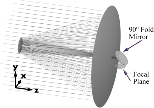
Fig. 2. An example Cassegrain telescope system with a primary mirror at F/1.2, a Cassegrain focus of F/8, and a 90° fold mirror in the F/8 converging beam. The 90° fold mirror is folded about the x-axis. The primary mirror has a clear aperture of 2.4 meters. The operating wavelength is 800 nm. All three mirrors are coated with aluminum. x and y define the coordinates for incident polarization states.

Fig. 3. Reflection coefficients for the amplitude (a) and the phase (b) of a complex wave upon reflection at angle of incidence θ° between 0° and 90° for a bare aluminum mirror at 800 nm wavelength are shown. In (b), ϕrs and ϕrp are the reflected phase for s and p-polarized light. The green vertical line highlights the reflection phase at 45°. The red and blue lines show the corresponding slope of ϕrs and ϕrp at the 45° incident angle.
2.1. The Fresnel Coefficients and Fresnel Aberrations
When a plane wave is incident on a metal reflector, the radiation's electric and magnetic fields drive the charges in the metal, which undergo a small oscillation at optical frequencies. These accelerating charges give rise to the reflected beam. The response of the charges, and thus the reflected beam, depends on the orientation of the electric field. The reflection process is a linear and can be completely described by the reflection of the s-component and p-component separately.
Figure 4 provides the notation to express the Fresnel equations which calculate the polarization content of the reflected beam. The complex refractive index N = n + ik, has imaginary part k and real part n. The values of n and k are given in optical materials handbooks (Palik 1961). Given the angle of incidence θ0 and the incident medium refractive index N0, the angle of refraction in medium 1 is found using Snell's law: N0 sin θ0 = N1 sin θ1, where N1 and θ1 and θ0 are defined in Figure 4. From  , the angle θ1 is

which for metals is a complex angle. The reflectivity for p-polarized light, polarized parallel to the plane of incidence, is given by the Fresnel coefficient for p-polarized light (Azzam et al. 1987),


Fig. 4. An incident ray propagating in medium (0) of index N0 reflects from a metal mirror of index N1 at angle θ° at point O. The metal medium N1 is assumed optically thick and the energy entering the metal is rapidly absorbed. The Fresnel reflection coefficients rs and rp separately describe the reflectance for the s and p-polarized components. The electric field vector for the light polarized in the s direction is out of the paper, normal to the plane of incidence, and the direction vector for the light polarized in the p direction is parallel to the plane of incidence.
Similarly the reflectivity rs for the s-polarized light, polarized perpendicular to the plane of incidence is

The amplitude reflection components in Figure 3a describe the relative amplitude of the reflected light. The fraction of reflected flux is the amplitude squared, |rs|2 and |rp|2, which for normal incidence is 0.9322 = 0.87. The remainder of the light's energy is lost to resistance from the charges moving through the metal, heating the reflector in the process. In Figure 3a, the s-reflectance is seen to be greater than the p-reflectance, leading to diattenuation. The variations of |rs| and |rp| with angle cause amplitude aberrations. For s-polarized light, the wavefront is brighter at larger angles of incidence while for p-polarized light the wavefront is dimmer. This apodization has a small effect on the image quality. The difference between |rs|2 and |rp|2 indicates that the reflectors act as weak polarizers. The polarization-dependent reflectance is characterized by the diattenuation D,

Metallic reflection acts as a weak polarizer, called a diattenuator after the two attenuations. Diattenuation varies from zero when all polarization states have the same reflectance or transmission (as with ideal retarders or nonpolarizing interactions) to one for ideal polarizers. When unpolarized light, such as starlight, is incident, the diattenuation is equal to the DoP of the exiting light. Due to the diattenuation, light incident in states different from s and p have some fraction of the energy coupled into the orthogonal polarization, and these orthogonally polarized components have an important role in the image formation that will be highlighted later.
Figure 3b shows the phase change on reflection, which is different for the s and p-polarizations. This phase change is a contribution the mirrors to the wavefront aberrations of the system. The phase shift δ between the s and p-reflected beams upon reflection is the retardance,

Since s and p at interfaces are linearly polarized states, this retardance is referred to linear retardance. Linear retardances with their fast axes aligned add; linear retardances with perpendicular fast axes subtract. In general the retardance of a sequence of retarders is simulated through the multiplication of Jones or Mueller matrices. Sequences of linear retardances at arbitrary orientations have elliptically polarized eigenvectors (fast and slow axes).
The polarization aberration changes the polarization state of a small fraction of the light, and as described later, that component changes the intensity and polarization distribution of the image, which can be an important factor in high contrast and resolution imaging. For small diattenuation (dimensionless) or small retardance (radians), the maximum fraction F of light which can be coupled into the orthogonal polarization state occurs for light at 45° to the diattenuation axis or retardance axis and both have the same quadratic form for F,

These equations are readily derived using the Mueller calculus by placing a diattenuator or retarder oriented at 45° between crossed polarizers and evaluating the Taylor series for the transmitted flux.
To generate scaling rules for polarization aberration, approximate forms for the diattenuation (eq. [4]) and retardance (eq. [5]) due to the Fresnel coefficients are presented in the appendix. For the two on-axis mirrors, these Fresnel coefficients have been expanded as even quadratic equations about normal incidence (eq. [A7]); for the fold mirror, these coefficients have been expanded as linear equations about the axial ray (eq. [A8]).
The phases in Figure 3b are important; they are polarization-dependent contributions to the wavefront aberration. They are perturbations to the wavefront which change depending on the metal or coating applied (McGuire & Chipman 1991). Since the fold mirror is in a converging beam, the nonzero slopes of the s and p-phases are both important and have been highlighted in Figure 3b. These slopes cause linear phase shifts, which shift the locations of the X and Y-polarized components from the geometrical image location, and since the slopes are different with opposite slopes, these components move in different directions by a small fraction of the Airy disk radius. Wavefront correction (e.g., adaptive optics) can flatten the slope of the phase through angle. Since the slopes are different for s and p-phases, wavefront correction can only correct either the s-polarized wavefront or the p-polarized wavefront, but not both simultaneously. This effect is discussed further in § 2.6 and in § 5 (design rules 8, 9, and 10).
2.2. Polarization Aberration
The polarization aberration of the example telescope of Figure 2 will first be examined from maps of diattenuation and retardance and then as a Jones matrix representation at the exit pupil. The diattenuation contributions from the three mirror elements are shown in the first three panels of Figure 5. The fourth panel in Figure 5 shows the cumulative diattenuation for the entire telescope as viewed looking into the exit pupil from the image plane. Each line inside the circle shows the diattenuation magnitude and the orientation of the maximum transmission axis at a point in the pupil. The primary and secondary mirrors (the first two panels in Fig. 5) produce rotationally symmetric, tangentially oriented diattenuation with a magnitude that increases quadratically from the center of the pupil.5 The fold mirror introduces a horizontally oriented diattenuation with a linear and cubic variation along the vertical axis. The cumulative diattenuation map shown on the right is predominantly linear from top to bottom. Polarization aberration functions which closely fit these diattenuation maps are discussed in the appendix.
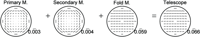
Fig. 5. Diattenuation maps for each mirror element (first three panels) and the cumulative diattenuation for the entire telescope (last panel). The length of each line is proportional to the value of the diattenuation and the orientation of the line shows the axis of maximum transmission for a point in the pupil. The key in the lower right corner of each panel shows the scale of the largest diattenuation. For this example telescope, the dominant source of diattenuation is the 90° fold mirror.
The aluminum's retardance introduces a polarization-dependent phase contribution to the OPL differently for the s and p-components of the light. Retardance aberration thus represents a difference in the metal coating's wavefront aberration contribution as experienced by orthogonal polarization states. Figure 6 shows the individual surface contributions to the retardance aberration in the first three panels and the cumulative retardance aberration through the system in the last panel. Each line shows the retardance magnitude and fast axis orientation at a grid of locations in the beam. The primary and secondary mirrors produce a rotationally symmetric tangentially oriented fast axis, which increases quadratically from the center, while the fold mirror introduces retardance with a vertically oriented fast axis. The fold mirror has a linearly varying retardance increasing from the bottom to the top of the pupil. Since the fold mirror has the largest retardance, the resultant retardance for the entire telescope shown on the right is similar to the fold mirror retardance with contributions from the primary and secondary mirrors. The cumulative linear retardance map (the fourth panel of Fig. 6) is primarily a constant retardance, with a linear variation from bottom to top, and a variation of retardance orientation from left to right. The cumulative retardances are shown as linear retardances (lines) but because the three individual weak retardances in the first three panels are not strictly parallel or perpendicular, the fast and slow axes of the retardances in the last panel are slightly elliptical; however, the ellipticity, which has a maximum value of 0.0047, is much smaller than would be visible at this scale. Similarly the diattenuation becomes slightly elliptical when the axes are not aligned, and in the map of Figure 5 has a maximum ellipticity of 0.011.

Fig. 6. Retardance maps for each mirror element (first three panels) and the cumulative retardance for the entire telescope (last panel). The length of each line is proportional to the value of the retardance and the orientation of the line shows the fast axis. The key in the lower right corner of each of the four panels shows the scale of the largest retardance in radians. This figure shows that the dominant source of retardance at the exit pupil for the telescope of Fig. 2 is the 90° fold mirror (third panel).
Polarization aberration functions which approximate these retardance maps are discussed in the appendix. Constant retardance is a constant difference in the wavefront aberration, a "piston" between polarization states; it changes polarization states but piston does not degrade image quality. The linear variation of retardance indicates a difference in the wavefront aberration tilt, X- and Y-polarizations get different linear phases, and so their images are shifted from the nominal image location by different amounts (see the end of § 2.2).
The spatial variation of the telescope's diattenuation (fourth panel of Fig. 5) and retardance (fourth panel of Fig. 6) is a low order variation which can be characterized by simple polynomials (see
Unlike conventional astigmatism, which on-axis would likely be caused by a cylindrical deformation in a mirror, this coating-induced astigmatism arises from the primary and secondary mirror's retardance defocus and is tied to the polarization state of the light. Coating-induced astigmatism rotates with the polarization state, whereas for a cylindrical deformation, the astigmatism would rotate with the mirror and not with the polarization state. For unpolarized light, the coating-induced astigmatic image is the average over the PSF of all polarization components, which is also the sum of the PSF for any two orthogonal components. So the astigmatism which is seen in a single incident polarization state, such as X-polarized, when added to the astigmatism for Y-polarized light, where the astigmatism is rotated by 90°, forms a radially symmetric PSF, which is slightly larger than the unaberrated image. Inserting a polarizer will reveal the astigmatism in any particular polarization component. More information on retardance defocus and the associated astigmatism in Cassegrain telescopes is found in Reiley & Chipman (1994).
2.3. The Jones Pupil
Each ray through the optical system has an associated Jones matrix, which describes the polarization change, the diattenuation and retardance, for that ray path (Jones 1941). The polarization aberration function is the set of Jones matrices expressed as a function of pupil coordinates and object coordinates (McGuire & Chipman 1990). The set of Jones matrices for a specified object point is called the Jones pupil, and has the form of a Jones matrix map over the pupil (Ruoff & Totzeck 2009). The Jones pupil is represented by the 2 × 2 Jones matrix, which contains complex components with amplitude A(x,y) and phase ϕ(x,y) at each point in the pupil (x,y),

For the X-polarized incident field at the entrance pupil, the term AXX is the amplitude of JXX at point (x,y) of the X-polarized field at the exit pupil. Also, for the X-polarized incident field at the entrance pupil, AYX is the amplitude at point (x,y) of light coupled from X into the Y-polarized field at the exit pupil. The term ϕYX, the complex argument of JXX, is the phase shift from the X-polarized incident field to the X-polarized exiting field due to the metal reflections. Similarly ϕYX is the phase shift for the X-polarized field coupled into the Y-polarized field. The field from a single point in object space maps into the 2 × 2 Jones matrix shown on the right of equation (7). Similarly, the right column of J describes the effects for the Y-polarized incident field.
The Jones pupil is calculated using the algorithms of geometrical optics (ray-tracing) augmented with polarization ray tracing. During the ray trace, the angle of incidence and orientation of the plane of incidence are evaluated at each ray intercept, and the Fresnel equations are used to calculate the s and p-reflection coefficients, as plotted in Figure 3. These coefficients are used to generate a polarization matrix for the ray intercept, such as a Jones matrix (Yun, Crabtree, & Chipman 2011). The OPL contributions are summed for each ray segment to determine the geometrical phase in the exit pupil. This is repeated for a grid of rays to calculate the geometrical wavefront aberration function. "Geometrical" here refers to the calculation of OPL, as determined by conventional ray tracing, without the influence of instrumental polarization. The polarization matrices are multiplied for each ray intercept from the entrance pupil through the exit pupil to determine the amplitudes in each polarization and the contributions of the metallic reflections to the overall phase.
A coordinate system must be chosen for the description of Jones matrices. The choice of the orthogonal basis is arbitrary. Here it is simplest to decompose the incident plane waves into a component parallel to our fold mirror's rotation axis, horizontal or X-polarized, and a vertical or Y-polarized component. The result of all flux and PSF calculations is independent of the orthogonal basis chosen.
A polarization ray trace was performed on the example telescope of Figure 2 and the values of the Jones pupil elements, given by equation (7), are displayed in Figure 7, which is color coded to show the amplitude and phase variations across the exit pupil. This Jones pupil is very close to the identity matrix times ∼0.806; the 0.806 accounts for average reflection losses from aluminum. Deviations from the identity matrix occur because the aluminum mirrors are weakly polarizing. Equation (A2) contains a closed form approximation to this Jones pupil.

Fig. 7. Values of the Jones pupil elements, given by eq. (7), are displayed as color-coded images to show variation across the exit pupil. The four images in (a) show the amplitude as a function of pupil position and the four images in (b) show the phase. Since AXY and AXY are highly apodized, their diffraction patterns are significantly larger than images associated with the diagonal terms. A scale appears to the right of each box: units are amplitude for (a) and phase in radians for (b). The phase of a complex number changes by π when the amplitude passes through zero. This causes the phase discontinuities in ϕXY and ϕYX.
The JXX and JYY diagonal elements contain different amount of polarization aberrations. The overall JXX amplitude is about 5% larger than the overall JYY amplitude because of the s and p-reflection difference at 45° shown in Figure 3a. This will cause the x-polarized image to be about 9% brighter than the y-polarized image. From the amplitude images of the Jones pupil in Figure 7a is close to the identity matrix, only a small fraction of the light has its polarization changed. The off-diagonal JXY and JYX elements show the polarization coupling between orthogonal polarizations. This polarization crosstalk has relatively low amplitude compared to the diagonal elements. The amplitudes AXX and AYY are nearly constant (< 2%), but the AXY and AYX are highly apodized, showing a Maltese cross pattern (dark along x and y-axes) shifted downwards.
The phases of the four elements in the Jones pupil, shown in the Figure 7b, represent contributions to the wavefront aberration function from the aluminum mirrors. The Fresnel phase changes are different for the s and p-components leading to different wavefronts for these two components. Since the on-axis geometrical wavefront aberration of the telescope is zero, the phase variation across the pupil are wavefront contributions from the mirror coatings. ϕXX, the wavefront aberration function of the telescope illuminated with x-polarized light and analyzed with an x-analyzer, has an overall linear variation of about 0.008 waves with an additional deviation, which is primarily astigmatism. The diagonal elements ϕXX and ϕYY have a different wavefront tilt between the ϕXX and ϕYY wavefronts. The source of this tilt difference is shown in Figure 3b, where it is seen that about a 45° angle of incidence, the slopes of the phase change are different for s- incident polarized light than for p- polarized light at the fold mirror. If the Fresnel phases were linear about 45°, only tilt would be introduced. The deviations from linear introduce higher order aberrations including small amounts of astigmatism (from quadratic deviation), coma (from cubic deviation), and other aberrations.
2.4. Amplitude Response Matrix
In conventional scalar image formation calculations, the amplitude response function is calculated as the Fourier transform of the exit pupil function. This electric field distribution is then squared to obtain the point spread function (Goodman 2004). To evaluate the image formed by systems with polarization aberration, McGuire & Chipman (1990) introduced a Jones calculus version of the amplitude response function named the Amplitude Response Matrix (ARM),

where  is a spatial Fourier transform over each of the Jones pupil elements. For a plane wave incident on the telescope with Jones vector E, the amplitude and phase of the image is given by the matrix multiplication, ARM·E. The ARM for the 3-mirror telescope of Figure 2 is shown in Figure 8. Table 1 summarizes the system and the parameters most relevant to the imaging calculations.

Fig. 8. The absolute value of the amplitude of the 2 × 2 ARM at an on-axis field point is shown for the example telescope of Fig. 2 normalized by the peak of the XX-component.
 |
The ARM's diagonal elements are close to the well-known Airy disk pattern, but are slightly larger due to the aberrations in ϕXX and ϕYY. Each is slightly astigmatic. Their centroids are slightly shifted due to the differences in their tilt. The off-diagonal elements have much lower amplitudes and contain interesting structure, mostly due to the fold mirror. We refer to these off-diagonal PSF images as the ghost PSFs.
For unpolarized illumination, the incident X- and Y-polarizations are incoherent with respect to each other. So the output components ARMXX (X in X out) and ARMYX (X in Y out) are coherent with each other but incoherent with ARMXY and ARMYY. So for unpolarized illumination, the two output X-components in the ARM are incoherent with respect to each other, as are the two output Y-components. So the point spread function for an unpolarized source has four additive components I = IX + IY = (|ARMXX|2 + |ARMXY|2) + (|ARMYX|2 + |ARMYY|2). The polarization structure of the generic telescope PSF is explored further in the next section.
2.5. Mueller Matrix Point Spread Matrices
The distribution of flux and polarization in the image of an incoherent point source, such as a star, can be described with a 4 × 4 Mueller matrix Point Spread Matrix (PSM), the Mueller matrix generalization of the PSF (McGuire & Chipman 1990). This PSM is calculated by the transformation of the ARM's Jones matrices into Mueller matrix functions (Goldstein 2010; Gil 2007; Chipman 2009). The Mueller matrix representation of polarization properties is familiar to most astronomers who make or work with astrophysical measurements of the four Stokes parameters (Gehrels 1974; Hovenier et al. 2005). The example telescope's PSM, calculated from the ARM (Fig. 8), is shown in Figure 9.

Fig. 9. The 4 × 4 point spread matrix (PSM) (left) operates on an example X-polarized incident beam with Stokes parameters (1, 1, 0, 0) (middle) to calculate the point spread function. The resultant polarization distribution is a 4 × 1 Stokes image (right) with components (IX, QX, UX, VX). The subscript X represents Stokes parameters resultant from X-polarized incident light. The normalized magnitude of each matrix element is shown on each vertical scale. The UX image indicates a small variation of polarization orientation, while VX indicates small variations of ellipticity. The red box on the left (m00, m10, m20, m30) is the resultant Stokes parameter image (I, Q, U, V) for a collimated beam of unpolarized incident light, such as an unpolarized star.
The contribution of each of the 16 elements varies across the PSM and changes depend on the incident Stokes parameters. Hence, each element of the matrix is shown with its contribution and appears as miniature PSF's with different shapes. An example of PSM measurements is found in McEldowney et al. (2008).
The PSF for unpolarized illumination is described by the Stokes parameter image in the first column (m00, m10, m20, m30) inside the red rectangle. Since m10, m20 and m30 are not zero, the PSF of an unpolarized star is not unpolarized. In this example, the Q component's 4.7 × 10⁻² contribution mostly arises from the diattenuation of the fold mirror, which is reflecting more 0° (s-polarized) light than 90° (p-polarized) polarized light. The U component (at 4.36 × 10⁻³) is mostly due to the diattenuation contributions at 45° and 135° from the primary and secondary seen in the first two panels in Figure 5. The ellipticity (from the V component) arises when weakly polarized light reflected from the primary and secondary interacts with the retardance from the fold mirror. The spatial variations of Q, U, and V introduce polarization fluctuations in the region of the diffraction rings. Figure 10 maps the DoP in these zones. Such polarization fluctuations in the PSF of a star are clearly a concern when measuring the polarization of exoplanets and debris disks.

Fig. 10. The DoP variation throughout the point spread function of an unpolarized object. Regions with intensity below 0.0008 of the peak have been removed due to noise and are shown in black.
Figure 9 contains a graphical equation describing the 4 × 4 PSM operating on an X-polarized incident beam (represented by the 4 × 1 matrix) which yields a 4 × 1 Stokes image, (IX, QX, UX, VX), as represented by the right-most term in the equation. For an unpolarized collimated incident beam, the resulting Stokes image is contained in the first column of the PSM, shown inside the red box. The m10 element describes the ∼9% DoP for the image of the unpolarized source. The m20 element describes small variations of linear polarization orientation within the PSF while m30 characterizes even smaller ellipticity variations.
The light coupled into orthogonal components has a significant impact on the outer portions of the PSF because they arise from the highly apodized Jones pupil components AXY and AYX as shown in Figure 7a. To see this, compare the PSF arising from JXX and JYX. These PSF terms are calculated using the resultant Stokes image components on the right side of Figure 9 as:

The two terms in equation (9), IXX and IYX, are compared in Figure 11 where it is seen that the peak of IYX is about 10-5 of IXX. This "ghost PSF" should be very important in imaging applications that require contrast ratios of 10-8 or greater.

Fig. 11. PSF of IXX and IYX calculated from eq. (9) are shown normalized to the peak of IXX.
Figure 12 shows the irradiance along an x-axis cross-section through the two PSFs in log 10 scale at the plane drawn through the two images shown in Figure 11. This ghost PSF has its light spread away from the center. In Figure 12, the Airy disk's zeros of IXX are not at the same location as the zeros for the cross-coupled term IYX. Thus, the zeros of IXX are washed out by the light leakage from the nonzero IYX. The point spread function IYX cannot be corrected by wavefront compensation for either the XX or YY-components alone because most of the image spread is due to IYX's apodization (Fig. 7). A linear Polaroid placed at the image plane can pass IXX and remove IYX, but will still pass the other ghost IXY, and thus will not correct for this polarization aberration.

Fig. 12. (a) Cross sections through the log 10 PSF image for IXX and IYX between -1 and +1 arcsecond along the x-direction. The solid and dashed curves show IXX and IYX, respectively. Note that at the first three minima of IXX (dark rings in the Airy disk) are close to the angles for the local maxima of the IYX curve. On the average the polarization coupled IYX flux shifted by about 10-4 below IXX. (b) Image plane for IYX shown in log 10 contour with its scale on the right ranging from -2.4 to -4.1, normalized to the peak intensity of IXX. The superposed green circles show the location of the first and second Airy dark ring of IXX.
The shape of IYX shows that the IX and QX Airy disks are not exactly on top of each other. The image plane irradiance distribution for the IYX term sits beneath the Airy diffraction pattern characteristic of the IXX term. Figure 12a shows a slice normal to the axis at the RMS best focus through the PSF for IXX and for IYX in Figure 11. Figure 12b shows a high-dynamic range image of the irradiance across the focal plane in the vicinity of the core of the PSF for IYX. The concentric green circles superposed on Figure 12b shows the first and second zeros of the Airy diffraction pattern of IXX. These dark rings overlay regions with nonzero IYX.
The right column in Figure 9, (IX, QX, UX, VX), is the Stokes parameter PSF for the X-polarized component of an incident beam. The flux of this component is IX = IXX + IYX. Similarly, the PSF IY for a Y-polarized incident beam is calculated by multiplying the Stokes parameters (1, -1, 0, 0) to the PSM, and IY = IYY + IXY. Finally the PSF for unpolarized incident light is (IX + IY)/2 which can also be calculated by multiplying the unpolarized Stokes parameters (1, 0, 0, 0) to the PSM.
This demonstrates that for unpolarized starlight passing into a "generic" optical system like that shown in Figure 2, the PSF is the sum of two nearly Airy diffraction patterns, IXX and IYY, plus two secondary or "ghost" PSFs, IYX and IYX, which originates from system's polarization cross-talk, the off-diagonal elements in the Jones pupil.
The Jones pupil, ARM, and PSM can be calculated in other basis sets than x and y. Here x and y are aligned parallel and perpendicular to the fold mirror's s-state. The resulting Jones pupil and ARM for other bases are found by Cartesian rotation of the matrices of Figures 7 and 8. The overall flux distributions, I = IX + IY, for an unpolarized source or point source of arbitrary polarization are unchanged by such a change of basis. Similarly, the PSM is rotated by the same rotation operation as Mueller matrices, and again the net flux for any source polarization is unchanged; the corresponding Stokes images are just rotated versions of the ones presented above. The advantage of the x and y basis chosen here is that the off-diagonal elements IXY and IYX have their smallest values in this basis. As the basis set rotates or becomes elliptical, the scale of these off-diagonal image components increases rapidly and quickly approach Airy disks due to the coupling between bright diagonal elements and weak off-diagonal elements from the rotation operation. Thus, the fold mirror's s and p-basis (our x and y) is best basis for viewing the value and functional form of the ghost PSF components for the example system of Figure 2.
2.6. Location of the PSF Images
Consider a Stokes imaging polarimeter located before the telescope of Figure 2's focal plane measuring the PSF of an unpolarized star as a Stokes image. The PSFs for the X-polarized, IX = IXX + IYX, and Y-polarized light, IY = IXY + IYY, at the focal plane are very close in form to the classical Airy diffraction pattern because the polarization-induced wavefront aberration, ϕXX and ϕYY in Figure 7, is less than 8 milliwaves, and the amplitude apodization is less than 0.015. But these two PSF images are not exactly superposed, the peaks of IX and IY are displaced from each other by 0.625 mas. The PSF cross-section through the maxima of IX, IY, and IX–IY (the star's Stokes Q image), are shown in Figure 13. The shift between the IX and IY PSFs arises from the difference in slopes of the s- and p-phases in the Fresnel coefficients (Fig. 3b, red and blue tangent lines), which is the cause of the overall linear variations in ϕXX and ϕYY. Their difference Q = IX - IY is sheared from IX and IY by 5.8 mas, as shown in Figure 13, and is due to the shift between IX and IY. These PSF's shifts and PSF's ellipticities are listed in Table 2 for a single 45° fold mirror before the focal plane. The ellipticity of the PSF image was calculated by fitting an ellipse to the PSF at the half power points.

Fig. 13. The cross-section profiles of the IX and IY PSF images, one for each polarization and the profile of their difference are shown in red and blue in arcseconds from the center of the PSF. The black line shows Stokes Q image, the difference between the two PSFs.
 |
In astronomical applications involving the precise measurement of the location of the centroid of the PSF, distortions of the shape of the PSF are important. Most systems incorporate multiple folds, for example in Goullioud et al. (2014) and Witzel et al. (2011). These relay optics with multiple folds may increase the shear between PSF's polarization components. The variation of linear phase across the pupil, as seen in Figure 3, is approximately linear, thus the shear between polarization components is linear in the F/#. As Clark & Breckinridge (2011) showed, across the FOV, variations of PSF ellipticity and orientation are expected from polarization aberration.
The Fresnel polarization aberrations, unless corrected, may affect our ability to characterize exoplanets using space telescopes. At least two mitigation approaches have been suggested. These are discussed in § 4.
2.7. Multiple Fold Mirrors
Many astronomical instruments require multiple fold mirrors, which often rotate with respect to each other. Consider the telescope in Figure 14 with five-fold mirrors. In the altitude axis and azimuth axis configuration shown, these folds are all coplanar, and the s-polarized light reflecting from the first mirror is s-polarized at all five mirrors; similarly p-polarized light at the first mirror is p-polarized at all five mirrors. For this configuration, the retardances for the axial ray at all five mirrors add. For general configurations where rotations have been performed on the axes, Jones matrices for a ray at all five mirrors need to be multiplied, and a data reduction step (Lu & Chipman 1994) performed to determine the retardance.

Fig. 14. A generic telescope layout with five-fold mirrors, showing all reflecting in the same plane (coplanar) such that the p-polarized light from the first fold is p-polarized at the other four mirrors, causing the polarization effects to all add, which is the worst case for the polarization from multiple fold mirrors. Rotations, such as about the altitude axis or azimuth axis, can cause a reduction in this overall polarization.
From Figure 3 and equation (5), we see that the retardance is defined as the absolute value of the difference in the phase between s and p-polarized light. The retardance adds cumulatively. The angles of incidence of the axial ray shown in Figure 14 are all equal to 45° (deviate the light by 90°) and therefore, the retardance for collimated rays at the exit pupil will be 5 times the retardance of a single 90° deviation reflection. By equation (6), 25 times the light would be coupled into orthogonal polarization states compared to a single-fold mirror. Also, the diattenuation, given in equation (4), increases approximately five-fold in the configuration of Figure 14.
Recall the linear variation of retardance induces a small spatial shift between the XX and YY PSM components. When the five coplanar mirrors in Figure 14 are reflecting a 0.06 numerical aperture (na) converging beam (F/8, as in the system of Fig. 2) in sequence, the converging ray from the left side of the secondary has a greater angle of incidence at the first, second, and fifth fold mirrors than the axial ray, and a smaller angle of incidence at the third and fourth mirrors. The linear variation of retardance across the pupil is the sum of the linear variations of the five individual coplanar mirrors. Each fold mirror has a retardance pattern corresponding to Figure 6 (third panel for fold mirror). So the linear variation of retardance adds for mirrors one, two, and five, and subtracts for mirrors three and four. The overall linear variation would be unchanged, and be the same as the linear variation of the single-fold mirror of Figure 2. The separation between the XX and YY-polarized images (discussed in the second paragraph of § 2.2), which depends on this linear retardance variation, would be unchanged. But the ghost PSFs would be 25 times greater than those shown in Figures 11 and 12. This all changes once the telescope is steered about the azimuth axis and altitude axis. Such general cases of sequences of fold mirrors in noncollimated beams can always be analyzed by polarization ray tracing. Lam & Chipman (2014) contains additional information on the polarization aberrations for sequences of fold mirrors.
3. Polarization Wavefront Division
It has been suggested that dividing the wavefront into two polarized beams and transmitting each of these to their own focal plane with their own adaptive optical system may alleviate some polarization aberration problems (Balasubramanian et al. 2011). This polarization wavefront division approach has the substantial disadvantage of doubling the number of flight hardware optical components and, in theory reduces the signal-to-noise ratio (S/N) by at least a factor of 0.7, but can improve overall image quality.
Consider an incoherent unpolarized source such as a star. The output of the generic telescope of Figure 2 divides at the polarizing beam splitter (PBS) shown in Figure 15 sending the linearly polarized X-component into one coronagraph at focal plane and the Y-component into another. The light from the JXX and JXY elements of the Jones pupil, shown in Figure 7, will exit into one path and JYX and JYY exit into the other path. The elements JXX and JXY are incoherent and their wavefronts do not interfere.

Fig. 15. Telescope system image plane showing the field, Ein input to a PBS, for example a Wollaston prism, which divides the wavefront by polarization. The image in one polarization passes to a coronagraph with its adaptive optics (A/O) system in path 1 and the image in the orthogonal polarization passes to a second coronagraph with its A/O system in path 2.
A simple example might help visualize the situation. Consider two nearly collimated beams from two different incoherent sources superposed and exiting a beam splitter. Both wavefronts have the same polarization state. One is slightly converging with positive defocus and one is slightly diverging with negative defocus. Their wavefronts are superposed but do not add into a single wavefront. An adaptive optics system could compensate one wavefront or the other, but not both.
So the adaptive optics in the first path of Figure 15 can perform wavefront compensation on JXX but the weak ghost PSF from JXY will remain aberrated. The adaptive optics in the second path can perform wavefront compensation on JYY but the weak ghost PSF from JYX will remain. Now the two principal PSF components are corrected, which is an improvement over the correction of only one component or their average. The overall image quality is improved from the single channel, single adaptive optic system. The issue of the weak but spatially larger contributions from the JXY and JYX ghosts remains. The ARM shown in Figure 8 for the example system provides the values of the polarization components relative to the XX-component. Their value shows that the ARMXY cross coupling "ghost" is 270 times less than ARMXX, and ARMYX is 260 times less than ARMYY.
4. Polarization Aberration Mitigation
Optical designers have a variety of methods to change the polarization aberrations of any particular optical system (Maymon & Chipman 1992). It is beyond the scope of this article to elaborate on these methods in detail. Fresnel and coating-induced polarization aberrations tend to be of small magnitude with low order functional variation (constant, linear, quadratic, etc.) (Chipman 1989a, 1989b). The following summarizes several mitigation approaches:
- 1.Reducing angles of incidence: Since the diattenuation and retardance are quadratic in the angle of incidence for modest angles, reducing the largest angles of incidence can significantly reduce polarization aberration. For example, fold mirror angles can be reduced or the F/# of mirrors and lenses reduced.
- 2.Reducing coating polarization: The optical-coating prescriptions for antireflection coatings of lenses and reflection-enhancing coatings of mirrors provide design degrees of freedom (thicknesses and materials) to adjust the diattenuation and retardance. In our experience, these coating prescriptions can be adjusted to moderately reduce the polarization properties, but cannot zero out diattenuation or retardance for substantial angle and wavelength ranges. The surfaces of antireflection coated lens typically have one third or less the diattenuation of uncoated lens surfaces, providing great benefit. The reflection-enhancing coatings for mirror often increase the retardance and diattenuation of metal mirrors in some wavebands.
- 3.Compensating polarization elements: Polarization aberrations can be introduced in several ways. Simply placing a (spatially uniform) weak polarizer (diattenuator) and a weak retarder in the system could zero out the polarization aberration at one point in the pupil, leaving overall polarization aberrations smaller. A spatially varying diattenuator and retarder with polarization magnitude approximately equal to the cumulative diattenuation and retardance of Figures 5 and 6 but orthogonally oriented, would nearly eliminate the polarization aberration. Such a polarization plate could be considered as the matrix inverse of the Jones pupil in Figure 7. Such correction plates might be fabricated from liquid crystals polymers with spatially varying magnitude and orientation of diattenuation or retardance, similar to the vortex retarders used in coronagraphy (Clark & Breckinridge 2011; McEldowney, Shemo, & Chipman 2008; Mawet et al. 2009). Wedged, spherical, and aspherical crystalline elements or element assemblies can provide a wide variety of compensating polarization aberrations (Chowdhury et al. 2004). Since polarization aberrations of telescopes and fold mirrors tend to be small, spatially varying anisotropic thin films, which can only provide small retardances, could provide another path toward compensation (Hodgkinson 1998).
- 4.Crossed fold mirrors: Fold mirrors tilted about opposite axes, such that the p-polarized light exiting one mirror is s-polarized on the second, have a compensating effect for both diattenuation and retardance (Maymon & Chipman 1992; McClain et al. 1992). A linear variation of polarization about the zero will still remain across the pupil.
- 5.Compensating optical elements: The diattenuation of lenses has the opposite sign (greater p-transmission) than the diattenuation of mirrors. Thus, including lenses would reduce the diattenuation from the primary and secondary mirrors in the example system. Similarly, sets of coatings might be selected to have opposite retardance contributions. Despite several concerted attempts, the author (Chipman) has not been able to change the sign of the diattenuation or retardance of an antireflection or reflection-enhancing coating over a useful spectral bandwidth. In practice, this approach has never been very successful.
Considering these mitigation approaches, when novelty, fabrication issues, scattering, tolerances, and risk are balanced against the small magnitude of the polarization aberration, these cures can easily become worse than the problem.
To design optical systems, typically a merit function is defined to characterize the wavefront and image quality, and an optimization program adjusts the system's constructional parameters to find acceptable configurations. (1) If polarization ray tracing parameters are included in the merit function, parameters such as diattenuation and retardance, the optimizer can balance the polarization aberrations against the wavefront aberrations and other constraints, pushing the solutions toward reduced polarization aberration. (2) Similarly, if the coating and polarization element constructional parameters are included in the optimization, the optimizer can explore the coating design space and polarization element configuration to find compensation schemes. For example, overcoated layers on aluminum will modify the polarization shown in Figure 3. These two steps are complicated, but advanced users can apply these methods, often through the use of the optical design program's macro languages, to evaluate polarization mitigation strategies listed above.
5. Scaling Relations And Design Rules For Polarization Aberrations
To assist in the analysis of the polarization aberrations and polarization image defects of other optical systems, a set of design rules are presented to show how the polarization aberration of the example telescope changes for different F/#, fold mirror angles, and coatings. These design rules provide guidance regarding the first two mitigation strategies: (1) reducing angles of incidence and (2) reducing coating polarization. A closed form expression for the example telescope's Jones pupil is developed in equation (A2) in the appendix based on six retardance and diattenuation aberration terms. These aberration terms are comparatively simple because they only involve constant, linear, and quadratic variations of diattenuation and retardance. These terms can be reevaluated for variations of the optical prescription of the example system with different coatings to show how the image defects scale based on these changes to the optical system, such as fold mirror angles and coating substitutions. Similar equations can be developed for more general optical systems.
The polarization aberrations of many systems can be described with only six polarization aberration terms, J1,J2,...J6, listed in Table 3. The Pauli matrices σ are defined in equation (A1). The six polarization aberration terms are plotted in Figure 16. These terms have functional forms similar to the wavefront aberrations piston (constant polarization), tilt (linearly varying from the origin and changing sign at the origin), and defocus (quadratically varying from the origin). This expansion is also mathematically similar to describing the diattenuation and retardance each with the first three Zernike polynomials (Ruoff & Totzeck 2009). Each of these three aberration forms occurs once for diattenuation with real coefficients. d0, d1, and d2, and once for retardance with imaginary coefficients Δ0, Δ1, and Δ2. The equations of Table 3 are first order expansions assuming small coefficients. For example, for retardance piston, the exact form of a retarder with retardance Δ1 is (σ0 cos Δ1/2 + iσ1 sin Δ1/2) which becomes (σ0 + iσ1Δ1/2) for Δ1 ≪ 1.
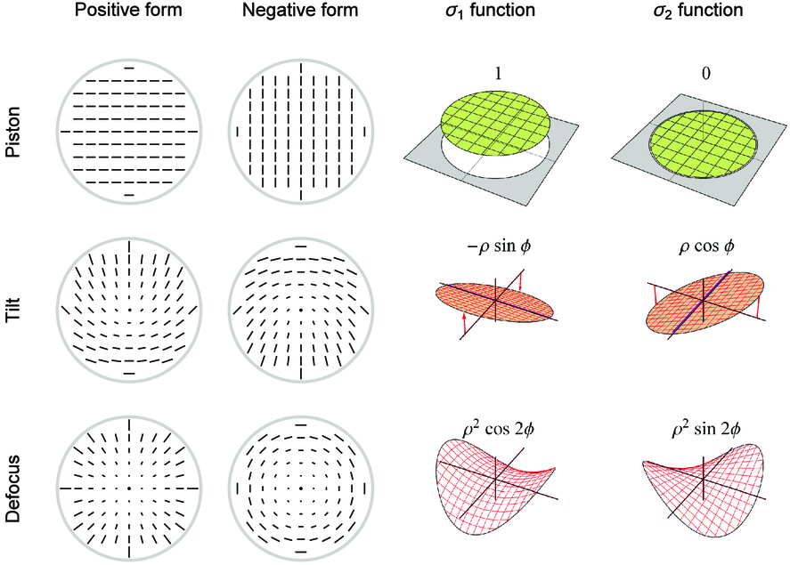
Fig. 16. Representation of the three forms of second-order polarization aberration, (top) piston aberration, J1 and J4, (middle) tilt aberration, J2 and J5, and (bottom) defocus aberration, J3 and J6. The first column shows a pupil map of the magnitude and orientation of the form. The second column shows the form with an opposite sign, which rotates all orientations by 90°. The right two columns show the decomposition of the aberration into σ1 and σ2 Pauli matrix components.
 |
The coefficient values for the example system of Figure 2 with aluminum coatings are listed in Table 4 in the appendix on the last row (the entry for Fig. 7). These polarization aberration coefficients depend on the diattenuation and retardance behavior of the mirror coatings, which can be parameterized for the purposes of the polarization aberration expansion by linear and quadratic equations (eqs. [A7] and [A8] in the appendix) with fitting coefficients a0, a1, and a2 for coating diattenuation and b0, b1, and b2 for coating retardance. The coefficients for the example optical system's aluminum coating at 800 nm are tabulated in Table 5.
 |
 |
A list of design rules will be considered based on the behaviors of the aberrations of Figure 16 for the following list of the example telescope's image defects:
- 1.Diattenuation at the center of the pupil,
- 2.Retardance at the center of the pupil,
- 3.The PSF shear between the XX and YY-components,
- 4.The polarization-dependent astigmatism, and
- 5.The fraction of light in the ghost PSF in components XY and YX.
The diattenuation at the center of the pupil corresponds to the diattenuation piston term J1 with magnitude d0. This arises only from the fold mirror; the primary and secondary mirrors do not contribute diattenuation at the center of the pupil. The coefficient d1 is close to the value of the average diattenuation, averaging over the pupil. J1 is primarily responsible for the 9% difference in the flux transmitted to the focal plane between the incident X and Y-polarized components. Unpolarized light has a ∼4% DoP when incident at the focal plane. This is typically calibrated out when using focal plane Stokes polarimeters. The magnitude of d0 only depends on the diattenuation at the fold mirror evaluated at the axial ray's angle of incidence θ3 (for surface 3, 45° in this case). This leads to two design rules for the average diattenuation.
Design rule 1: The average diattenuation (diattenuation piston value) characterized d0 by is quadratic in the fold mirror angle θ3.
Design rule 2: The diattenuation piston value, d0, is linear in the coating parameter a0 defined in equations (A7) and (A8) in the appendix. If a0(λ) is calculated for a coating as a function of wavelength, the spectral variation of the average diattenuation will be proportional to a0(λ). If the aluminum is overcoated with silicon monoxide or some other material, the quadratic variation of diattenuation can be calculated at normal incidence to compare the resulting average diattenuation between coatings.
The retardance at the center of the pupil corresponds to the retardance piston term J4 with value Δ0. J4 also arises only from the fold mirror. The coefficient Δ0 is close to the value of the average retardance, averaging over the pupil. J4 does not change the polarization (Stokes parameters) of unpolarized light transiting the system, it only modifies polarized light. J4 introduces a constant phase difference between the X and Y-incident components; thus, J4 does not degrade the PSF. The value of Δ0 only depends on the retardance at the fold mirror evaluated at the axial ray's angle of incidence θ3. This leads to two more design rules.
Design rule 3: The retardance piston characterized by Δ0 is quadratic in the fold mirror angle θ3.
Design rule 4: Δ0 is linear in the coating parameter b0.
The diattenuation tilt J2 with magnitude d1 describes a linear variation of diattenuation across the pupil, corresponding to unpolarized light exiting with a smaller DoP at the bottom of the pupil and a larger DoP at the top of the pupil. J2 arises only from the fold mirror; the primary and secondary mirrors do not contribute. J2 causes the X-polarized input to be brighter at the top of the pupil becoming linearly dimmer toward the bottom of the pupil. Y-polarized input has the opposite variation. This apodization has a very small effect on the shape and structure of the XX and YY-PSFs, much smaller than the other polarization imaging defects treated in this article. J2 does contribute significantly to the off-diagonal Jones pupil elements JXY and JYX and thus to the brightness of the ghost PSFs, IXY and IYX. The value of d1 depends on the slope of the diattenuation a1 at the fold mirror evaluated at θ3 and on the range of angles at the fold mirror, characterized by the F/# in image space, F/8, or na = 0.06. This leads to the design rules for the diattenuation tilt J2.
Design rule 5: The diattenuation tilt characterized by d1 is linear in the angle θ3. This follows from the slope of a quadratic function, equation (A7), being linear.
Design rule 6: d1 is linear in the coating diattenuation slope parameter a1.
Design rule 7: d1 is also linear in the coating diattenuation quadratic parameter angle a2, which follows from the slope of a quadratic function being linear.
The retardance tilt J4 with value Δ1 describes a linear phase variation for the XX-polarized component and an opposite linear phase variation of for the YY-polarized component. This arises only from the fold mirror; the primary and secondary mirrors do not contribute. J4 is a very important term because it shifts the images of the XX and YY-components in opposite directions causing the overall PSF to become elliptical. J4 also contributes to the off-diagonal Jones pupil elements JXY and JYX and thus, to the brightness of the ghost PSFs, IXY and IYX. The value of Δ1 depends on the slope of the retardance at the fold mirror evaluated at θ3 and on the range of angles at the fold mirror, characterized by the numerical aperture. This leads to the design rules for the retardance tilt J4.
Design rule 8: The retardance tilt characterized by Δ1 is linear in the fold mirror angle θ3, which follows from the slope of a quadratic function being linear.
Design rule 9: The retardance tilt magnitude Δ1 is linear in the coating retardance slope parameter b1.
Design rule 10: The retardance tilt magnitude Δ1 is also linear in the coating retardance quadratic parameter b2, which follows from the slope of a quadratic function, b1, being linear in the quadratic parameter.
The diattenuation defocus term J3 with magnitude d2 describes a quadratic diattenuation variation from the center the pupil which is tangentially oriented. This arises primarily from the primary and secondary mirrors with a small contribution from the fold mirror. J3 causes the X-polarized input to exit brighter at the top and bottom of the pupil than the center and dimmer at the left and right sides. The effect on Y-polarization is rotated by 90° and the pupil is brighter on the left and right sides. This apodization has a very small effect on the shape and structure of the XX and YY-PSFs, much smaller than the other imaging effects treated in this article. J3 does contribute to the off-diagonal Jones pupil elements Jxx and Jyy and thus, to the brightness of the ghost PSFs IXY and IYX. The magnitude of d2 depends on the quadratic variation of the diattenuation about normal incidence a2, and on the angle of incidence of the marginal ray at the edge of the primary θ1 and secondary θ2 mirrors. This leads to the design rules for the diattenuation defocus J3.
Design rule 11: The diattenuation defocus characterized by d2 is quadratic in the sum of the marginal ray angles θ1 + θ2 assuming identical coatings, and thus is quadratic in the na, assuming the design F/# is scaled by just changing the entrance pupil diameter.
Design rule 12: The diattenuation defocus magnitude d2 is quadratic in the coating diattenuation quadratic parameter a2.
The retardance defocus term J6 with magnitude d2 describes a quadratic variation of retardance from the center the pupil which is tangentially oriented. This arises primarily from the primary and secondary mirrors with a small contribution from the fold mirror. J6 causes the X-polarized input exiting into X-polarized output to become astigmatic (Reiley & Chipman 1994). From the center, the phase is advanced quadratically along the x-axis, and delayed quadratically along the y-axis. For YY, this astigmatism is rotated by 90°. The effect on unpolarized light is like spinning the astigmatic PSF, the PSF is rotationally symmetric, but enlarged by the astigmatism. J6 also contributes to the off-diagonal Jones pupil elements JXX and JYY and thus, to the brightness of the ghost PSFs, IXY and IYX. The magnitude of d2 depends on the quadratic variation of the retardance about normal incidence b2, and on the angle of incidence of the marginal ray at the edge of the primary θ1 and secondary θ2 mirrors. This leads to the design rules for the retardance defocus J6.
Design rule 13: The retardance defocus characterized by Δ2, and thus the polarization-dependent astigmatism, is quadratic in the sum of the angles θ1 + θ2 assuming identical coatings, and thus is quadratic in the na if the design F/# is scaled by just changing the entrance pupil diameter.
Design rule 14: The retardance defocus magnitude Δ2 is quadratic in the coating retardance quadratic parameter b2.
Design rule 15: The maximum fraction of flux coupled into the orthogonal state for weak linear polarization elements is quadratic in the diattenuation and quadratic in the retardance, and occurs for incident light polarized at 45° to the diattenuation axis or retardance fast axis. This follows from equation (6).
The fraction FYX of the X-polarized incident light coupled into the ghost PSF image IYX depends on the tilt coefficients d1 and Δ1 and the defocus coefficients d2 and Δ2, but not the piston coefficients. This is also equal to the fraction FXY of the Y-polarized incident light coupled into the ghost PSF image IXY. This fraction is determined by integrating the magnitude squared of the complex off-diagonal elements of the Jones pupil over the pupil, as described in equation (A6), and depends quadratically on the coefficients d1, Δ1, d2, and Δ2. Analysis of the tilt aberrations leads to design rules for the fractions FXY and FYX.
Design rule 16: The fraction of the flux incident in either the X-polarization or the Y-polarization coupled into the orthogonal ghost images IYX (fraction FYX) or IXY (fraction FXY) depends quadratically on d1 and Δ1. Since d1 and Δ1 are linear in the angle θ3, FYX and FXY are quadratic in the fold mirror angle θ3. See design rules 5 and 8. FYX and FXY are also quadratic in the coating retardance slope parameters a1 and b1. See design rules 6 and 9. FXY and FYX are also quadratic in the coating diattenuation quadratic parameter a2. See design rules 7 and 10.
Analysis of the defocus aberrations leads to additional design rules for the fractions FYX and FXY. The diattenuation defocus, d2, and the retardance defocus, Δ2, is quadratic in the sum of the marginal ray angles θ1 + θ2 assuming identical coatings.
Design rule 17: The fractions FYX and FXY are fourth order in the sum of the marginal ray angles θ1 + θ2 assuming identical coatings, and thus fourth order in the na, assuming the design F/# is scaled by just changing the entrance pupil diameter. Thus, small decreases in F/# can yield large increases in ghost PSF brightness. See design rules 11 and 13.
Design rule 18: The fractions FYX and FXY are fourth order in the coating diattenuation quadratic parameter a2. See design rules 12 and 14.
Thus these design rules describe the scaling of the polarization aberration as the pupil size changes, F/# changes, coating prescription changes, and fold mirror angle changes. These relations only apply to the on-axis beam of optical configurations similar to Figure 2. The off-axis equations become considerably more complicated, but coronagraphs and other astronomical systems usually have small enough fields that the polarization aberration variation over the field is not significant, and therefore these design rules do not change over this system's practical field-of-view. As more fold mirrors or other components are added to this system, these polarization aberration equations need to be generalized to relate the polarization aberrations to the coating prescriptions and optical prescription. Lam & Chipman (2015) discussed polarization aberration reduction with two and four mirror combinations. Discussions of higher order polarization aberration terms can be found in McGuire & Chipman (1994a, 1994b), Ruoff & Totzeck (2009), and Sasian (2012, 2014).
6. Astronomical Effects Of Telescope Polarization Aberrations
6.1. Exoplanet Discovery and Characterization
The intensity of the ghost PSF is about one part in 10-4 of the two primary PSF images IXX and IYY and with spatial structure of much larger extent across the focal plane and with more structural complexity than the classical Fraunhofer scalar diffraction PSF. The exoplanet community needs to control the intensity PSF to a part in 10-10 or 10-6 of the magnitude below the intensity level for the ghost PSF image which has been calculated for the "typical" telescope system described here. The intensity and the structural complexity in this ghost PSF have the potential to disguise terrestrial exoplanets images and become a source of false positive discoveries and measurement errors. The "ghost" PSF overfills the image plane mask designed using scalar theory and will obscure exoplanet images. The presence of the ghost PSF and its intensity depend on the packaging configuration of mirrors and the physical optics properties of the highly reflective mirror coatings within the mechanical layout of the entire telescope/instrument optical system.
For example, Groff & Kasdin (2013), Carlotti et al. (2013), and Carlotti et al. (2011) design, build, and optimize image and pupil plane masks using scalar models of reflecting optical systems. These masks are now being developed for the new AFTA-WFIRST coronagraph. Our results here show that a modified system of stops and masks may be needed to optimize the WFIRST coronagraph mission for exoplanets.
6.2. Astrometry Errors
Astrometry is the measurement of the fundamental position of objects in the sky. Applications include determining the dynamics of the galaxy and calculating the orbital elements of gravitationally interacting bodies. Astrometric precision depends on the precise measurement of the intensity centroid of each point source within an ensemble of point sources across the FOV as mapped by the telescope system onto the focal plane. Typical measurements are to better than 1% of the size of the PSF to achieve an error in the ensemble of less than 0.1%. An inherent assumption is that the intensity centroid remains constant across the FOV. However, the contents of Table 2 shows that accurate modeling of the effects of instrumental polarization indicates centroid asymmetries of about 1%. At 800 nm wavelength, the full width at half max of the PSF image is about 70 mas. McArthur et al. (2011) report absolute parallaxes of select stares in the Hyades to errors near 0.2 mas for HST data; this is 0.2% of the FWHM for stellar PSF's at 500 nm from HST.
Astrometric reference stars are chosen to be at great distances so they appear fixed over long periods of time in relation to foreground objects. The light from these distant objects becomes partially polarized by interstellar matter, particularly, in the Galactic bulge region. The PSF image for partially polarized stars becomes asymmetric due to the polarization aberration. The magnitude and orientation of this asymmetry depends on the number of fold mirrors in the telescope and the bore sight orientation of the telescope. Astrometrists need to consider polarization aberrations as sources of measurement error.
7. Summary
Astronomical applications require high photometric accuracy, high contrast, and diffraction-limited performance. Polarization ray tracing is an important tool for assessing image quality. Most modern large aperture astronomical telescopes use low F/# primaries with several reflecting surfaces before the focal plane; the polarization aberration of these components can produce changes to the PSF of a magnitude comparable to the specifications of the current generation of coronagraphs and high-contrast imagers.
To highlight the issues, a polarization analysis of image quality was performed for a generic telescope, a 2.4 meter, F/1.2 primary mirror Cassegrain telescope with a single 45° fold mirror in front of the focal plane for an F/8 converging beam. We make the following summary observations:
- 1.The polarizing properties of the primary, secondary, and fold mirrors cause a difference in the wavefront aberrations (tilt, coma, astigmatism, spherical, etc.) between light polarized parallel and perpendicular to the fold mirror rotation axis (Fig. 6). If the number of high-angle reflections in the design increases, this difference can increase.
- 2.The fold mirror in converging light causes a shift between the PSFs for X- and Y-polarizations which elongates the overall PSF. The angle between the two PSFs depends on several factors: the number of fold mirrors, the deviation angle of the beams upon reflection, the mirror coatings (metal and dielectric over coating), and wavelength.
- 3.The X- and Y-polarizations show a difference in intensity transmittance, causing unpolarized sources to exit partially polarized into the instrument packages.
- 4.The telescope coatings cause polarization variations throughout the PSF, particularly into the diffraction rings, which may complicate polarization measurements of exoplanets and debris rings in coronagraphs.
- 5.Adaptive optics systems cannot simultaneously correct the wavefront aberrations of both polarizations. Coupling (leakage) of one polarization state into the other will limit the performance of the adaptive optics system. This coupling is characterized by the off-diagonal elements in the Jones pupil. Dividing the wavefront by polarization and using two adaptive optics systems improves the overall wavefront correction, while increasing system complexity and reducing the S/N.
- 6.For unpolarized light, the light from one polarization which is coupled into its orthogonal state is not coherent with respect to the orthogonal state, and forms a separate faint and much larger PSF superposed on the Airy diffraction pattern. If the number of high-angle reflections in the design is increased, and the mirrors s and p-planes are aligned, the intensity of this distorted "ghost" PSF can increase quadratically in the number of reflections to potentially affect measurements made using coronagraphs.
- 7.Geometrical ray trace optimizes geometric image quality by minimizing physical OPD. An analysis that also takes polarization into consideration at the image plane is needed to determine whether or not the wavefronts represented by those rays create an image of sufficient quality. The geometric (optical path difference) ray trace of an optical system can be ideal (as in the example telescope) but the polarization content of each ray may change enough across the wavefront to reduce image quality.
- 8.Several methods of mitigating polarization aberration can possibly reduce polarization aberrations, including configuring elements to balance polarization aberrations, such as the opposite contributions to diattenuation from lenses and mirrors, or the aberration reduction from "crossed mirrors", and polarization aberration compensators such as spatially variable retardance and diattenuation plates.
- 9.Design rules to partially mitigate the effects of internal polarization are discussed here and references to polarization mitigation device technology are given. These relations bring a machinery to bear on this optical system example comparable to the calculation of Seidel aberrations of lenses from the paraxial ray trace.
The following recommendations are made for future work in this area. For planned ground-based and space-based systems, vector-wave (polarization) ray tracing and physical optics analysis methods should be applied to model realistic telescope/coronagraph contrast limits with the thin films, adaptive optics, and opto-mechanical tolerances. All components need to be considered as potential polarization sources, including metal and dielectric thin films, optical filters, polarization analyzers, and dispersing elements. The beam needs to be sampled over the entire field-of-view, F/#, and beam deviation angles from gratings and rotating mirrors throughout the entire end-to-end optical telescope/instrument system to the focal plane. This work can be used to assess the need for polarization mitigation devices and begin their technology development. The importance of polarization aberrations to astrometric accuracy should be investigated with more representative optical system designs.
We acknowledge the prior support of the Science Foundation Arizona in the development of the polarization ray tracing program, Polaris-M, used in this analysis. We thank Karlton Crabtree for many contributions leading to this article. We also thank Dr. Keith Patterson who as a student at Caltech performed the initial numerical modeling of polarization in this optical system. We acknowledge the valuable comments provided by an anonymous reviewer.
Appendix:: Polarization aberration analysis
All the numerical results except in this appendix were calculated using polarization ray tracing, particularly the calculation of the Jones pupil in Figure 7. Ray tracing methods treat system performance and aberrations numerically as grids of OPLs, Jones matrices, and other values. In this appendix, an aberration theory analysis is used to describe the Jones pupil in Figure 7 in terms of simple closed form functions. This aberration theory is applied in § 5 to understand some design rules for polarization imaging defects which builds the scaling relationships between the magnitudes of defects and the constructional parameters of the optical system.
The diattenuation and retardance aberrations of many systems can be described with only six polarization aberration terms, J1,J2,...J6, listed in Table 3 of § 5. Detailed descriptions of these diattenuation and retardance aberrations are found in many references (Chipman 1987, 1989a, 1989b; Chipman & Chipman 1989; McGuire & Chipman 1994a, 1994b; Hanson 1988; Ruoff & Totzeck 2009). In general the diattenuation and retardance aberration of optical systems has lower order than the wavefront aberrations, and requires less terms in its aberration expansion for equivalent accuracy. The Jones matrix functions for these six polarization aberrations are defined in terms of the Pauli matrices, σ1, σ2, and σ3, augmented with the 2 × 2 identity matrix σ0,

Each aberration terms of the Jones matrix function is defined over the pupil using polar coordinates ρ, the normalized radial distance, and ϕ, the azimuth measured from the x-axis. The magnitude of each term is specified by an aberration coefficient d0, d1, and d2, for diattenuation terms, and Δ0, Δ1, and Δ2 for retardance terms. All six aberration coefficients are assumed to be much less than one. When these six terms are cascaded, and only the first order terms in σ1 and σ2 are kept, the result is the sum of the six aberration terms,

J is then combined with scalar terms for the wavefront aberration W(ρ,ϕ) and amplitude transmission A(ρ,ϕ) to complete the description of the Jones pupil,

The wavefront aberration W(ρ,ϕ) acquires small constant, linear, and quadratic terms from the Fresnel aberrations,

These are the wavefront aberrations piston w0, tilt w1, and, defocus w2. These are included in the approximation to the Jones pupil to bring the fit within 1%. Higher order wavefront aberrations, spherical aberration, coma, etc. are not generated in significant amounts at the three mirrors of the example, but are present at some level. Similarly, small polarization independent amplitude variations are generated from the Fresnel aberrations, and are expressed with coefficients a0, a1, and a2 as

Equation (A3) incorporating equation (A2) provides an accurate expression for the example telescope's Jones pupil. This equation with different coefficient values describes the Jones pupils of most camera lenses, microscope objectives, telescopes, and many other optical systems. It is a general purpose equation.
The fraction of incident flux incident in X or Y-polarization coupled into the orthogonal polarization state is found by integrating the off-diagonal element's (the σ2 term) magnitude squared |JYX|2 or |JXY|2 over the pupil and normalizing by π, the area of the pupil,

FXY is the fraction of the incident Y-polarized flux contained in the IXY image integrated over the image. FXY is quadratic in the tilt and defocus coefficients, so an order of magnitude reduction in these polarization aberrations reduces the ghost brightness by 2 orders of magnitude.
Next the aberration coefficients, d0, d1, d2, Δ0, Δ1, and Δ2, for the telescope of Figure 2 are examined. Each of these coefficients is the value of the diattenuation or retardance at the edge of the pupil for that specific term. These coefficients are related to the properties of the coating and the optical system's prescription. The description of the effects of each polarization aberration terms is found in § 5.
Table 4 lists the aberration coefficients for the retardance, diattenuation, amplitude, and wavefront for the Jones pupil of the telescope end-to-end from Figure 7. These coefficients were determined by curve fitting the coefficients of equation (A3) to the Jones pupil polarization ray trace data.
Note all of the polarization aberration coefficients are much less than one, so that the combination of terms in equation (A2) is an accurate representation for the cascaded polarization of the three elements. Figure 17 shows the Jones pupil of Figure 7 as approximated with the system aberration coefficients from Table 4. Along the y-axis and along a horizontal line below the x-axis, the amplitudes of the AXY and AYX terms change sign, so the phases ϕXY and ϕYX change by π along these lines. Figure 18 shows the small residual difference between the polarization ray trace result in Figure 7 and the polarization aberration expansion of Figure 17, which match to within 0.002 in amplitude, which is better than 0.2% of the average amplitude ∼0.8. Applying equation (A6), approximately 6 × 10⁻⁵ of the incident flux is coupled into the ghost PSFs by the off-diagonal elements of the Jones pupil.

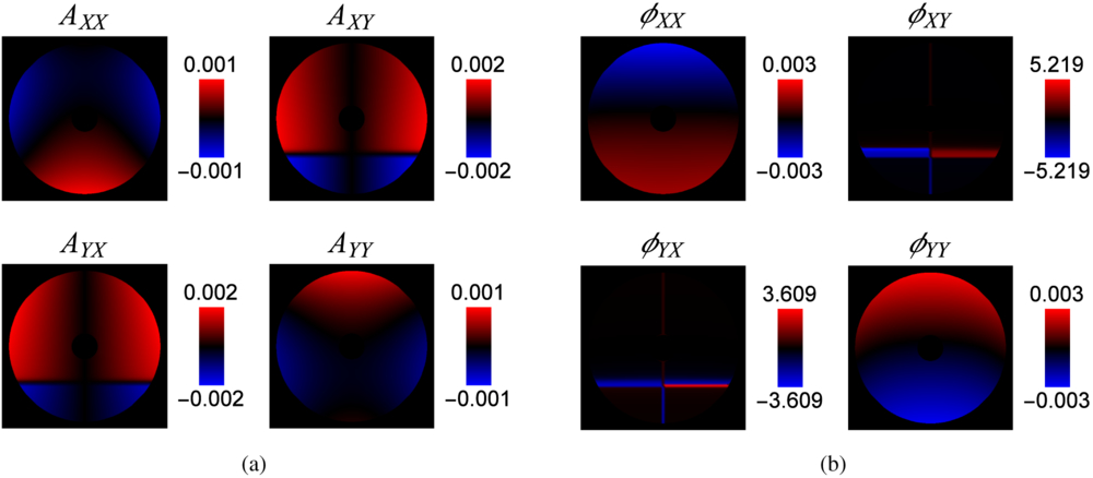
Fig. 18. The differences between the Jones pupil obtained by polarization ray tracing in Fig. 7 and the aberration expansion fit in Fig. 7 are small. In all of the plots, black represents a difference of zero, the fit generated by the aberrations expansion has the same value as the ray tracing data. This residual contains small contributions from polarization aberration terms of higher order than eq. (A2).
The phase and retardance values of Table 4 are provided in radians. They can be divided by 2π to express the aberration in waves. So for example, the aluminum coatings have contributed Δ1/2π ∼ 0.004 waves, or 4 milliwaves of polarization-dependent tilt. It is seen from the last line in Table 4 that the wavefront aberration contributions w1 and w2 contribute less than 5 milliwave of aberration in the present example.
Coating polarization can also be well approximated with simple polynomials for the purpose of developing scaling relationships and quickly estimating the effects of changing the system's coatings. For the on-axis mirrors, the coating diattenuation D(θ) and retardance δ(θ) functions are expanded about normal incidence in a quadratic function as

with second-order coefficients a2 for diattenuation and b2 for retardance. These quadratic fits about normal incidence are shown in Figures 19a and 20a for aluminum at 800 nm. For the aluminum fold mirror a first order expansion about the axial ray angle of incidence θ0 = 45° is used,

and the fits are shown in Figures 19b and 20b. The fit coefficients are tabulated in Table 5. Such Taylor series coefficients for aluminum are easily evaluated at other wavelengths to describe the polarization aberration as a function of wavelength. Similarly, numerical derivatives of coating design program output can be manipulated to get the Taylor series coefficients for other metals and for arbitrary multilayer coatings.

Fig. 19. (a) Aluminum diattenuation vs. angle of incidence with quadratic fit about 0° and (b) linear fit about 45°. Solid black lines are the exact diattenuation. Dashed black lines are the quadratic and linear fit of diattenuation; see Table 5. The solid green line in the right figure indicates angle of incidence of the axial ray and the dashed green lines indicate the range associated to na = 0.06 beams at the mirrors.

Fig. 20. (a) Aluminum retardance in radians vs. angle of incidence with quadratic fit about 0° and (b) linear fit about 45°. Solid black lines are the exact retardance. Dashed black lines are the quadratic and linear fit of retardance. The solid green line in the right figure indicates angle of incidence of the axial ray and the dashed green lines indicate the range associated to na = 0.06 beams at the mirrors.
Footnotes
- 5
When linear and quadratic, etc. are used throughout the manuscript, approximately linear and approximately quadratic are implied as is standard in aberration theory.